My Note
Notebook 6.2 Gradient descent
This notebook recreates the gradient descent algorithm as shown in figure 6.1.
Work through the cells below, running each cell in turn. In various places you will see the words “TODO”. Follow the instructions at these places and make predictions about what is going to happen or write code to complete the functions.
# import libraries
import numpy as np
import matplotlib.pyplot as plt
from matplotlib import cm
from matplotlib.colors import ListedColormap
# Let's create our training data 12 pairs {x_i, y_i}
# We'll try to fit the straight line model to these data
data = np.array([[0.03,0.19,0.34,0.46,0.78,0.81,1.08,1.18,1.39,1.60,1.65,1.90],
                 [0.67,0.85,1.05,1.00,1.40,1.50,1.30,1.54,1.55,1.68,1.73,1.60]])
# Let's define our model -- just a straight line with intercept phi[0] and slope phi[1]
def model(phi,x):
  y_pred = phi[0]+phi[1] * x
  return y_pred
# Draw model
def draw_model(data,model,phi,title=None):
  x_model = np.arange(0,2,0.01)
  y_model = model(phi,x_model)

  fix, ax = plt.subplots()
  ax.plot(data[0,:],data[1,:],'bo')
  ax.plot(x_model,y_model,'m-')
  ax.set_xlim([0,2]);ax.set_ylim([0,2])
  ax.set_xlabel('x'); ax.set_ylabel('y')
  ax.set_aspect('equal')
  if title is not None:
    ax.set_title(title)
  plt.show()
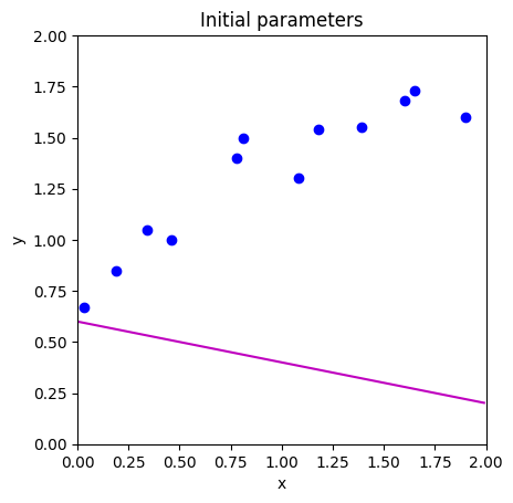
# Initialize the parameters to some arbitrary values and draw the model
phi = np.zeros((2,1))
phi[0] = 0.6      # Intercept
phi[1] = -0.2      # Slope
draw_model(data,model,phi, "Initial parameters")
def compute_loss(data_x, data_y, model, phi):
  # TODO -- Write this function -- replace the line below
  # First make model predictions from data x
  # Then compute the squared difference between the predictions and true y values
  # Then sum them all and return
  pred_y = 0
  loss = 0

  return loss
loss = compute_loss(data[0,:],data[1,:],model,np.array([[0.6],[-0.2]]))
print('Your loss = %3.3f, Correct loss = %3.3f'%(loss, 12.367))
Your loss = 0.000, Correct loss = 12.367
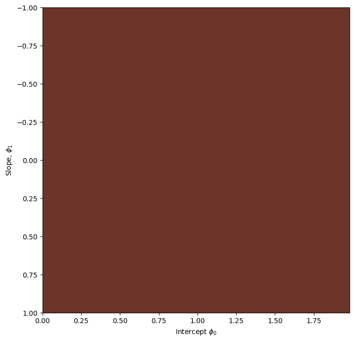
def draw_loss_function(compute_loss, data,  model, phi_iters = None):
  # Define pretty colormap
  my_colormap_vals_hex =('2a0902', '2b0a03', '2c0b04', '2d0c05', '2e0c06', '2f0d07', '300d08', '310e09', '320f0a', '330f0b', '34100b', '35110c', '36110d', '37120e', '38120f', '39130f', '3a1410', '3b1411', '3c1511', '3d1612', '3e1613', '3f1713', '401714', '411814', '421915', '431915', '451a16', '461b16', '471b17', '481c17', '491d18', '4a1d18', '4b1e19', '4c1f19', '4d1f1a', '4e201b', '50211b', '51211c', '52221c', '53231d', '54231d', '55241e', '56251e', '57261f', '58261f', '592720', '5b2821', '5c2821', '5d2922', '5e2a22', '5f2b23', '602b23', '612c24', '622d25', '632e25', '652e26', '662f26', '673027', '683027', '693128', '6a3229', '6b3329', '6c342a', '6d342a', '6f352b', '70362c', '71372c', '72372d', '73382e', '74392e', '753a2f', '763a2f', '773b30', '783c31', '7a3d31', '7b3e32', '7c3e33', '7d3f33', '7e4034', '7f4134', '804235', '814236', '824336', '834437', '854538', '864638', '874739', '88473a', '89483a', '8a493b', '8b4a3c', '8c4b3c', '8d4c3d', '8e4c3e', '8f4d3f', '904e3f', '924f40', '935041', '945141', '955242', '965343', '975343', '985444', '995545', '9a5646', '9b5746', '9c5847', '9d5948', '9e5a49', '9f5a49', 'a05b4a', 'a15c4b', 'a35d4b', 'a45e4c', 'a55f4d', 'a6604e', 'a7614e', 'a8624f', 'a96350', 'aa6451', 'ab6552', 'ac6552', 'ad6653', 'ae6754', 'af6855', 'b06955', 'b16a56', 'b26b57', 'b36c58', 'b46d59', 'b56e59', 'b66f5a', 'b7705b', 'b8715c', 'b9725d', 'ba735d', 'bb745e', 'bc755f', 'bd7660', 'be7761', 'bf7862', 'c07962', 'c17a63', 'c27b64', 'c27c65', 'c37d66', 'c47e67', 'c57f68', 'c68068', 'c78169', 'c8826a', 'c9836b', 'ca846c', 'cb856d', 'cc866e', 'cd876f', 'ce886f', 'ce8970', 'cf8a71', 'd08b72', 'd18c73', 'd28d74', 'd38e75', 'd48f76', 'd59077', 'd59178', 'd69279', 'd7937a', 'd8957b', 'd9967b', 'da977c', 'da987d', 'db997e', 'dc9a7f', 'dd9b80', 'de9c81', 'de9d82', 'df9e83', 'e09f84', 'e1a185', 'e2a286', 'e2a387', 'e3a488', 'e4a589', 'e5a68a', 'e5a78b', 'e6a88c', 'e7aa8d', 'e7ab8e', 'e8ac8f', 'e9ad90', 'eaae91', 'eaaf92', 'ebb093', 'ecb295', 'ecb396', 'edb497', 'eeb598', 'eeb699', 'efb79a', 'efb99b', 'f0ba9c', 'f1bb9d', 'f1bc9e', 'f2bd9f', 'f2bfa1', 'f3c0a2', 'f3c1a3', 'f4c2a4', 'f5c3a5', 'f5c5a6', 'f6c6a7', 'f6c7a8', 'f7c8aa', 'f7c9ab', 'f8cbac', 'f8ccad', 'f8cdae', 'f9ceb0', 'f9d0b1', 'fad1b2', 'fad2b3', 'fbd3b4', 'fbd5b6', 'fbd6b7', 'fcd7b8', 'fcd8b9', 'fcdaba', 'fddbbc', 'fddcbd', 'fddebe', 'fddfbf', 'fee0c1', 'fee1c2', 'fee3c3', 'fee4c5', 'ffe5c6', 'ffe7c7', 'ffe8c9', 'ffe9ca', 'ffebcb', 'ffeccd', 'ffedce', 'ffefcf', 'fff0d1', 'fff2d2', 'fff3d3', 'fff4d5', 'fff6d6', 'fff7d8', 'fff8d9', 'fffada', 'fffbdc', 'fffcdd', 'fffedf', 'ffffe0')
  my_colormap_vals_dec = np.array([int(element,base=16) for element in my_colormap_vals_hex])
  r = np.floor(my_colormap_vals_dec/(256*256))
  g = np.floor((my_colormap_vals_dec - r *256 *256)/256)
  b = np.floor(my_colormap_vals_dec - r * 256 *256 - g * 256)
  my_colormap = ListedColormap(np.vstack((r,g,b)).transpose()/255.0)

  # Make grid of intercept/slope values to plot
  intercepts_mesh, slopes_mesh = np.meshgrid(np.arange(0.0,2.0,0.02), np.arange(-1.0,1.0,0.002))
  loss_mesh = np.zeros_like(slopes_mesh)
  # Compute loss for every set of parameters
  for idslope, slope in np.ndenumerate(slopes_mesh):
     loss_mesh[idslope] = compute_loss(data[0,:], data[1,:], model, np.array([[intercepts_mesh[idslope]], [slope]]))

  fig,ax = plt.subplots()
  fig.set_size_inches(8,8)
  ax.contourf(intercepts_mesh,slopes_mesh,loss_mesh,256,cmap=my_colormap)
  ax.contour(intercepts_mesh,slopes_mesh,loss_mesh,40,colors=['#80808080'])
  if phi_iters is not None:
    ax.plot(phi_iters[0,:], phi_iters[1,:],'go-')
  ax.set_ylim([1,-1])
  ax.set_xlabel('Intercept $\phi_{0}$'); ax.set_ylabel('Slope, $\phi_{1}$')
  plt.show()
draw_loss_function(compute_loss, data, model)
# These are in the lecture slides and notes, but worth trying to calculate them yourself to
# check that you get them right.  Write out the expression for the sum of squares loss and take the
# derivative with respect to phi0 and phi1
def compute_gradient(data_x, data_y, phi):
    # TODO -- write this function, replacing the lines below
    dl_dphi0 = 0.0
    dl_dphi1 = 0.0

    # Return the gradient
    return np.array([[dl_dphi0],[dl_dphi1]])
# Compute the gradient using your function
gradient = compute_gradient(data[0,:],data[1,:], phi)
print("Your gradients: (%3.3f,%3.3f)"%(gradient[0,0],gradient[1,0]))
# Approximate the gradients with finite differences
delta = 0.0001
dl_dphi0_est = (compute_loss(data[0,:],data[1,:],model,phi+np.array([[delta],[0]])) - \
                    compute_loss(data[0,:],data[1,:],model,phi))/delta
dl_dphi1_est = (compute_loss(data[0,:],data[1,:],model,phi+np.array([[0],[delta]])) - \
                    compute_loss(data[0,:],data[1,:],model,phi))/delta
print("Approx gradients: (%3.3f,%3.3f)"%(dl_dphi0_est,dl_dphi1_est))
# There might be small differences in the last significant figure because finite gradients is an approximation
Your gradients: (0.000,0.000)
Approx gradients: (0.000,0.000)
def loss_function_1D(dist_prop, data, model, phi_start, search_direction):
  # Return the loss after moving this far
  return compute_loss(data[0,:], data[1,:], model, phi_start - search_direction * dist_prop)

def line_search(data, model, phi, gradient, thresh=.00001, max_dist = 0.1, max_iter = 15, verbose=False):
    # Initialize four points along the range we are going to search
    a = 0
    b = 0.33 * max_dist
    c = 0.66 * max_dist
    d = 1.0 * max_dist
    n_iter = 0

    # While we haven't found the minimum closely enough
    while np.abs(b-c) > thresh and n_iter < max_iter:
        # Increment iteration counter (just to prevent an infinite loop)
        n_iter = n_iter+1
        # Calculate all four points
        lossa = loss_function_1D(a, data, model, phi, gradient)
        lossb = loss_function_1D(b, data, model, phi, gradient)
        lossc = loss_function_1D(c, data, model, phi, gradient)
        lossd = loss_function_1D(d, data, model, phi, gradient)

        if verbose:
          print('Iter %d, a=%3.3f, b=%3.3f, c=%3.3f, d=%3.3f'%(n_iter, a,b,c,d))
          print('a %f, b%f, c%f, d%f'%(lossa,lossb,lossc,lossd))

        # Rule #1 If point A is less than points B, C, and D then halve distance from A to points B,C, and D
        if np.argmin((lossa,lossb,lossc,lossd))==0:
          b = a+ (b-a)/2
          c = a+ (c-a)/2
          d = a+ (d-a)/2
          continue;

        # Rule #2 If point b is less than point c then
        #                     point d becomes point c, and
        #                     point b becomes 1/3 between a and new d
        #                     point c becomes 2/3 between a and new d
        if lossb < lossc:
          d = c
          b = a+ (d-a)/3
          c = a+ 2*(d-a)/3
          continue

        # Rule #2 If point c is less than point b then
        #                     point a becomes point b, and
        #                     point b becomes 1/3 between new a and d
        #                     point c becomes 2/3 between new a and d
        a = b
        b = a+ (d-a)/3
        c = a+ 2*(d-a)/3

    # Return average of two middle points
    return (b+c)/2.0
def gradient_descent_step(phi, data,  model):
  # TODO -- update Phi with the gradient descent step (equation 6.3)
  # 1. Compute the gradient (you wrote this function above)
  # 2. Find the best step size alpha using line search function (above)
  # 3. Update the parameters phi based on the gradient and the step size alpha.

  return phi
# Initialize the parameters and draw the model
n_steps = 10
phi_all = np.zeros((2,n_steps+1))
phi_all[0,0] = 1.6
phi_all[1,0] = -0.5
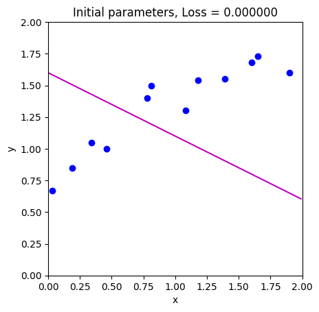
# Measure loss and draw initial model
loss = compute_loss(data[0,:], data[1,:], model, phi_all[:,0:1])
draw_model(data,model,phi_all[:,0:1], "Initial parameters, Loss = %f"%(loss))
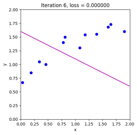
# Repeatedly take gradient descent steps
for c_step in range (n_steps):
# Do gradient descent step
phi_all[:,c_step+1:c_step+2] = gradient_descent_step(phi_all[:,c_step:c_step+1],data, model)
# Measure loss and draw model
loss = compute_loss(data[0,:], data[1,:], model, phi_all[:,c_step+1:c_step+2])
draw_model(data,model,phi_all[:,c_step+1], "Iteration %d, loss = %f"%(c_step+1,loss))
# Draw the trajectory on the loss function
draw_loss_function(compute_loss, data, model,phi_all)